¶ CSVファイルの読み込み
ここでは,(カンマ区切り)のCSVファイルを読み込むことを前提とする。以下サンプルファイル。
SampleData.csv
¶ CSVファイルの読み込みを確認
import pandas as pd

df = pd.read_csv(r'c:\Users\[ユーザー名]\Downloads\SampleData.csv') #rがないとエラーになる
print(df)

print(df.columns)
このままだと一行目が列名としてインポートされる。
runfile('C:/Users/[ユーザー名]/CSV_read_result.py', wdir='C:/Users/[ユーザー名]')
      0       0.1         1
0    10  0.173648  0.984808
1    20  0.342020  0.939693
2    30  0.500000  0.866025
3    40  0.642788  0.766044
4    50  0.766044  0.642788
..  ...       ...       ...
67  320 -0.642788  0.766044
68  330 -0.500000  0.866025
69  340 -0.342020  0.939693
70  350 -0.173648  0.984808
71    0  0.000000  1.000000

[72 rows x 3 columns]
Index(['0', '0.1', '1'], dtype='object')
¶ 列名がない場合のCSVファイルの読み込み
列名がない場合は"header=None"オプションを加える。
import pandas as pd

df = pd.read_csv(r'c:\Users\[ユーザー名]\Downloads\SampleData.csv', header=None)
print(df)

print(df.columns)
今度は1行目もデータとして認識された。
runfile('C:/Users/[ユーザー名]/CSV_read_result.py', wdir='C:/Users/[ユーザー名]')
      0         1         2
0     0  0.000000  1.000000
1    10  0.173648  0.984808
2    20  0.342020  0.939693
3    30  0.500000  0.866025
4    40  0.642788  0.766044
..  ...       ...       ...
68  320 -0.642788  0.766044
69  330 -0.500000  0.866025
70  340 -0.342020  0.939693
71  350 -0.173648  0.984808
72    0  0.000000  1.000000

[73 rows x 3 columns]
Int64Index([0, 1, 2], dtype='int64')
¶ CSVファイルの読み込み時に列名を割り当てる
列名を読み込み時に指定することもできる
import pandas as pd

df = pd.read_csv(r'c:\Users\[ユーザー名]\Downloads\SampleData.csv', names=('A', 'B', 'C')) #列名を配列で指定
print(df)

print(df.columns)
列名がついた。
runfile('C:/Users/[ユーザー名]/CSV_read_result.py', wdir='C:/Users/[ユーザー名]')
      A         B         C
0     0  0.000000  1.000000
1    10  0.173648  0.984808
2    20  0.342020  0.939693
3    30  0.500000  0.866025
4    40  0.642788  0.766044
..  ...       ...       ...
68  320 -0.642788  0.766044
69  330 -0.500000  0.866025
70  340 -0.342020  0.939693
71  350 -0.173648  0.984808
72    0  0.000000  1.000000

[73 rows x 3 columns]
Index(['A', 'B', 'C'], dtype='object')
¶ CSVファイルのグラフ化
#ライブラリインポート
import numpy as np
import matplotlib.pyplot as mp
import pandas as pd

#データ生成
#x = np.arange(256)
#y = np.random.randint(-100,100, size = 256)

df = pd.read_csv(r'C:\Users\[ユーザー名]\Downloads\SampleData.csv', names=('A', 'B', 'C')) #列名を配列で指定

#グラフ描画
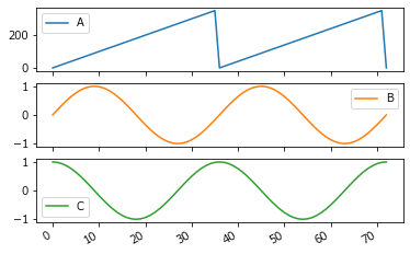
df.plot(subplots=True)
mp.show()                                                #グラフ表示
¶ 実行結果